Source
@article{hermans_2018_penalty,
    title={A penalty method based approach for autonomous navigation using nonlinear model predictive control},
    author={Hermans, Ben and Patrinos, Panagiotis and Pipeleers, Goele},
    journal={IFAC Conference on Nonlinear Model Predictive Control},
    volume={51},
    number={20},
    pages={234--240},
    year={2018},
    publisher={Elsevier}
}
(KU Leuven) | Elsevier | arXiv
TL;DR
Penalty method + General-shape obstacles
Flash Reading
- Abstract: MPC for handling obstacles of general shapes, through a quadratic penalty method and heuristics local-minima bypassing. Inner optimization problem is solved by the PANOC solver.
- Introduction: Challenges include (a) real-time constraints (gradient-based/first-order solvers are faster than second-order solvers, such as SQP and IP); (b) the way of formulating the problem affects the use of solvers. This paper combines the work in [1] with a penalty method framework. Some heuristics are used to further handle local minima. PANOC is used since it combines projected gradient and limited-memory quasi-Newton methods.
- Problem Formulation: Obstacle constraints are formulated as \(O=\{\bm{z}\in\mathbb{R}^{n_z}|h_i(\bm{z})>0,\,i=1,2,\ldots,m\}.\) The NMPC problem is formulated as (a. objective) tracking state and input references while (b. constraint) following the motion model, following action limits, and avoiding obstacles.
- Methodology: Construct a quadratic penalty function for the obstacle avoidance constraint. Solve the inner problem using the PANOC solver in the single-shooting fashion. Solve the outer problem using a penalty method.
Basics
- Obstacle constraints are formulated as \(O=\{\bm{z}\in\mathbb{R}^{n_z}|h_i(\bm{z})>0,\,i=1,2,\ldots,m\},\) where $h_i:\mathbb{R}^{n_z}\to\mathbb{R}$ are continuously differentiable functions with Lipschitz continuous gradients (value difference is bounded). The obstacle avoidance constraint ($\bm{z}\notin O$) can be written as \(\Psi(\bm{z}):=\prod_{i=1}^m[h_i(\bm{z})]_+ = 0.\) The notation $[\cdot]_+$ means $\max(0, \cdot)$. This means at least one of the $h_i(\bm{z})$ should be non-positive. In general, LICQ (Linear Independence Constraint Qualification) is not satisfied. Such a formulation can be used to model any polyhedral and ellipsoidal obstacles. For the quadratic penalty function $\tilde{\Psi}(\bm{z_k})=1/2\mu_k\Psi^2(\bm{z_k})$, where $k$ is the step index in the horizon and $\mu_k$ is the penalty parameter, the gradient is \(\nabla\tilde{\Psi}(\bm{z_k})=\mu_k\Psi(\bm{z_k})\nabla\Psi(\bm{z_k})=\mu_k\sum_{i=1}^m \left[ [h_i(\bm{z_k})]_+\prod_{j\neq i}[h_j(\bm{z_k})]_+^2 \nabla h_i(\bm{z_k}) \right] .\)
Key Points
Optimization Problem based on Penalty Method
The final optimization problem (single-shooting) is formulated as \(\begin{align*} \min_{\bm{u}_{1:N} \in U_{1:N}} & J_N(\bm{q}_N) + \sum_{k=0}^{N-1} J_k(\bm{q}_k, \bm{u}_k) + \frac{1}{2}\sum_{k=0}^{N-1} \sum_{i=1}^m \mu_{i,k} \Psi^2_i(\bm{z}_k), \\ \text{s.t. } & \bm{q}_{k+1} = f(\bm{q}_k, \bm{u}_k) \end{align*}\)
Penalty Method
The objective function depends on the penalty term, thus can be written as $\mathcal{L}(\bm{u}|\bm{\mu})$. The process of the penalty method is
Input: Initial guess '$\bm{u}_0$', penalty parameter '$\mu_0$'.
while (not converged) do: # Outer loop
    Solve the problem and get '$\bm{u}^*$'. # Inner loop
    Update the penalty parameter '$\mu$'.
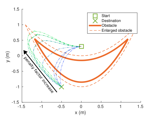
An increasing penalty parameter has a better chance to converge to the target, while a fixed high penalty parameter may lead to convergence to a local minimum.
Issues with Penalty Method
If the penalty parameter is too high, the problem may become ill-conditioned (vanishing and exploding gradients). PANOC uses an estimate of the Lipschitz constant of the objective to determine the step size, which linearly increases with the penalty parameter. Therefore, the penalty factor needs to be capped to stay within a reasonable range. However, this leads to no guarantee of finding a feasible solution.
Heuristics for Local Minima Bypassing
- To avoid collision, if the obstacle cost is not smaller than a threshold within a certain number of time steps, an emergency stop is triggered.
- (If the agent gets stuck) Use grid-based A* algorithm to find an intermediate waypoint to bypass the local minima.
References
- [1] Embedded nonlinear model predictive control for obstacle avoidance using PANOC, ECC 2018. Online.
Extension
First-Order vs Second-Order Optimization Solvers
| Method / Solver | Type | Derivative Used | Reference / Link |
|---|---|---|---|
| FISTA | First-order | Gradient only | Beck & Teboulle (2009) |
| ADMM | First-order | Gradient only | Boyd et al. (2011) |
| Chambolle–Pock | First-order primal-dual | Gradient only | Chambolle & Pock (2011) |
| PANOC | First-order + quasi-Newton | Gradient only + limited-memory | Stella et al. (2017) |
| Proximal Gradient | First-order | Gradient only | Parikh & Boyd (2013) |
| OSQP | First-order splitting | Gradient only | Stellato et al. (2020) |
| SQP (SNOPT) | Second-order | Gradient + Hessian | Gill et al. (2005) |
| IPOPT | Second-order (Interior Point) | Gradient + Hessian | Wächter & Biegler (2006) |
| Numerical Optimization Book | Reference book | Gradient + Hessian (for SQP & IP) | Nocedal & Wright (2006) |
- First-Order Methods: Use gradients only, faster per iteration, scalable to large problems.
- Second-Order Methods (SQP, IP): Use gradients + Hessians, more accurate per iteration but computationally heavier.